Tests Supplementing ANOVA
Learning Objectives
- Compute Tukey HSD test
- Describe an interaction in words
- Describe why one might want to compute simple effect tests following a significant interaction
Tests Supplementing ANOVA
- The null hypothesis tested in a one-factor ANOVA is that all the population means are equal
- Stated more formally,
H0: μ1 = μ2 = ... μk
k is the number of conditions
- When the null hypothesis is rejected, then all that can be said is that at least one population mean is different from at least one other population mean
- The methods described in the sections on All Pairwise Comparisons and on Specific Comparisons for doing more specific tests apply here
- Keep on mind that these tests are valid whether or not they are preceded by an ANOVA.
Main Effects
- As shown below, significant main effects in multi-factor designs can be followed up in the same way as significant effects in a one-way designs
- Table below shows the data from an imaginary experiment with three levels of Factor A and two levels of Factor B.
| A1 | A2 | A3 | Marginal Means | |
|---|---|---|---|---|
| B1 | 5 | 9 | 7 | 7.08 |
| 4 | 8 | 9 | ||
| 6 | 7 | 9 | ||
| 5 | 8 | 8 | ||
| Mean = 5 | Mean = 8 | Mean = 8.25 | ||
| B2 | 4 | 8 | 8 | 6.50 |
| 3 | 6 | 9 | ||
| 6 | 8 | 7 | ||
| 8 | 5 | 6 | ||
| Mean = 5.25 | Mean = 6.75 | Mean = 7.50 | ||
| Marginal Means | 5.125 | 7.375 | 7.875 | 6.79 |
- Table below shows the ANOVA Summary Table for these data
- The significant main effect of A indicates that, in the population, at least one of the marginal means for A is different from at least one of the others.
| Source | df | SSQ | MS | F | p |
|---|---|---|---|---|---|
| A | 2 | 34.333 | 17.17 | 9.29 | 0.0017 |
| B | 1 | 2.042 | 2.04 | 1.10 | 0.3070 |
| AB | 2 | 2.333 | 1.167 | 0.63 | 0.5431 |
| Error | 18 | 33.250 | 1.847 | ||
| Total | 23 | 71.958 | 3.129 |
Tukey HSD test
The Tukey HSD can be used to test all pairwise comparisons among means in a one-factor ANOVA as well as comparisons among marginal means in a multi-factor ANOVA.
The formula for the equal-sample-size case is shown below.
 Mi and Mj are marginal means
MSE is the mean square error from the ANOVA
n is the number of scores each mean is based upon
- For this example, MSE = 1.847 and n= 8 because there are eight scores at each level of A
- The probability value can be computed using the Studentized Range Calculator
- The degrees of freedom is equal to the degrees of freedom error
- For this example, df = 18
- The results of the Tukey HSD test are shown in Table 3
- The mean for A1 is significantly lower than the mean for A2 and the mean for A3
- The means for A2 and A3 are not significantly different.
| Comparison | Mi - Mj | Q | p |
|---|---|---|---|
| A1 - A2 | -2.25 | -4.68 | 0.0103 |
| A1 - A3 | -2.75 | -5.73 | 0.0021 |
| A2 - A3 | -0.50 | -1.04 | 0.7456 |
Specific comparisons among means are also carried out much the same way as shown in the relevant section on testing means
The formula for L is
 ci is the coefficient for the ith marginal mean
Mi is the ith marginal mean
For example, to compare A1 with the average of A2 and A3, the coefficients would be 1, -0.5, -0.5
L = (1)(5.125) + (-0.5)(7.375) + (-0.5)(7.875) = -2.5
To compute t, use:
 = -4.25
MSE is the mean square error from the ANOVA
n is the number of scores each marginal mean is based on (eight in this example)
- The degrees of freedom is the degrees of freedom error from the ANOVA and is equal to 18
- Using the Online Calculator, we find that the two-tailed probability value is 0.0005
- Therefore, the difference between A1 and the average of A2 and A3 is significant.
Important issues concerning multiple comparisons and orthogonal comparisons are discussed in the Specific Comparisons section in the Testing Means chapter.
Interactions
- The presence of a significant interaction makes the interpretation of the results more complicated.
- Since an interaction means that the simple effects are different, the main effect as the mean of the simple effects does not tell the whole story
- This section discusses how to describe interactions, proper and improper uses of simple effects tests, and how to test components of interactions
Describing Interactions
- A crucial step first step in understanding a significant interaction is constructing an interaction plot
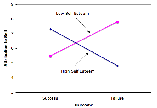
- Figure 1 shows an interaction plot from data presented in the section on Multi-factor ANOVA.
- The second step is to describe the interaction in a clear and understandable way
- This is often done by describing how by describing how the simple effects differed
- Since this should be done using as little jargon as possible, the word "simple effect" need not appear in the description
- An example is as follows:
The effect of Outcome differed depending on the subject's self esteem.
The difference between the attributions to self following success and attributions to self following failure was
larger for high-self-esteem subjects (mean difference = 2.50)
than for low-self-esteem subjects (mean difference = -2.33).
- No further analyses are helpful in understanding the interaction since the interaction means only that the simple effects differ
- The interaction's significance indicates that the simple effects differ from each other, but provides no information about whether they differ from zero.
- If neither simple effect is significant, the conclusion should be that the simple effects differ, and that at least one of them is not zero.
- However, no conclusion should be drawn about which simple effect(s) is/are not zero.
- Another error that can be made by mistakenly accepting the null hypothesis is to conclude that two simple effects are different because one is significant and the other is not
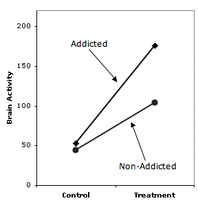
- Consider the results of an imaginary experiment in which the researcher hypothesized that addicted people would show a larger increase in brain activity following some treatment than would non-addicted people
- In other words, the researcher hypothesized that addiction status and treatment would interact
- The results shown in Figure 2 are very much in line with the hypothesis
- However, the test of the interaction resulted in a probability value of 0.08, a value not quite low enough to be significant at the conventional 0.05 level
- The proper conclusion is that the experiment supports the researcher's hypothesis, but not strongly enough to allow a firm conclusion.
Simple Effect Tests
- It is not necessary to know whether the simple effects differ from zero in order to understand an interaction because the question of whether simple effects differ from zero has nothing to do with interaction except that if they are both zero there is no interaction
- It is not uncommon to see research articles in which the authors report that they analyzed simple effects in order to explain the interaction
- However, this is not a correct since an interaction does not depend on the analysis of the simple effects.
- However, there is a reason to test simple effects following a significant interaction
- Since an interaction indicates that simple effects differ, it means that the main effects are not general
- In the made-up example, the main effect of Outcome is not very informative, and the effect of outcome should be considered separately for high- and low-self-esteem subjects.
- As will be seen, the simple effects of Outcome are significant and in opposite directions: Success significantly increases attribution to self for high-self-esteem subjects and significantly lowers attribution to self for low-self-esteem subjects
- This is a very easy result to interpret.
- What would the interpretation have been if neither simple effect had been significant?
- On the surface, this seems impossible: How can the simple effects both be zero if they differ from each other significantly as tested by the interaction?
- The answer is that a non-significant simple effect does not mean that the simple effect is zero: the null hypothesis should not be accepted just because it is not rejected
- If neither simple effect is significant, the conclusion should be that the simple effects differ, and that at least one of them is not zero.
- However, no conclusion should be drawn about which simple effect(s) is/are not zero.
Another error that can be made by mistakenly accepting the null hypothesis is to conclude that two simple effects are different because one is significant and the other is not. Consider the results of an imaginary experiment in which the researcher hypothesized that addicted people would show a larger increase in brain activity following some treatment than would non-addicted people. In other words, the researcher hypothesized that addiction status and treatment would interact. The results shown in Figure 2 are very much in line with the hypothesis. However, the test of the interaction resulted in a probability value of 0.08, a value not quite low enough to be significant at the conventional 0.05 level. The proper conclusion is that the experiment supports the researcher's hypothesis, but not strongly enough to allow a firm conclusion.
Unfortunately, the researcher was not satisfied with such a weak conclusion and went on to test the simple effects. It turned out that the effect of Treatment was significant for the Addicted group (p = 0.02) but not significant for the Non-Addicted group (p = 0.09). The researcher then went on to conclude that since there is an effect of Treatment for the Addicted group but not for the Non-Addicted group, the hypothesis of a greater effect for the former than for the latter group is demonstrated. This is faulty logic, however, since it is based on accepting the null hypothesis that the simple effect of Treatment is zero for the Non-Addicted group just because it is not significant.
Components of Interaction (optional)
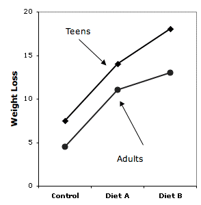
Figure 3 shows the results of an imaginary diet on weight loss. A control group and two diets were used for both overweight teens and overweight adults.
The difference between Diet A and the Control diet was essentially the same for teens and adults whereas the difference between Diet B and Diet A was much larger for the Teens than it was for the Adults. Over one portion of the graph the lines are parallel whereas over another portion they are not. It is possible to test these portions or components of interactions using the method of specific comparisons discussed previously. The test of the difference between Teens and Adults on the difference between Diets A and B could be tested with the coefficients shown in Table 4. Naturally, the same consideration regarding multiple comparisons and orthogonal comparisons apply to comparisons involving components of interaction that apply to other comparisons among means.
| Age Group | Diet | Coefficient |
|---|---|---|
| Teen | A | 1 |
| Teen | B | -1 |
| Adult | A | -1 |
| Adult | B | 1 |
Questions


