R - Forecasting

Approaches to Forecasting

• ARIMA (AutoRegresive Integrated Moving Average)
• ETS (Exponential smoothing state space model)

We will discuss how those methods work and how to use them.

Forecast package overview

 # Install Libraries
 install.packages("forecast")
 library("forecast")
 
 rawdata <- read.table("http://training-course-material.com/images/1/19/Sales-time-series.txt",h=T)
 rawdata$Date <- as.Date(rawdata$Date)
 head(rawdata)
 plot(rawdata)
 
 # Using build in ts object
 sts <- ts(rawdata$Sales,start=2001,frequency=12)
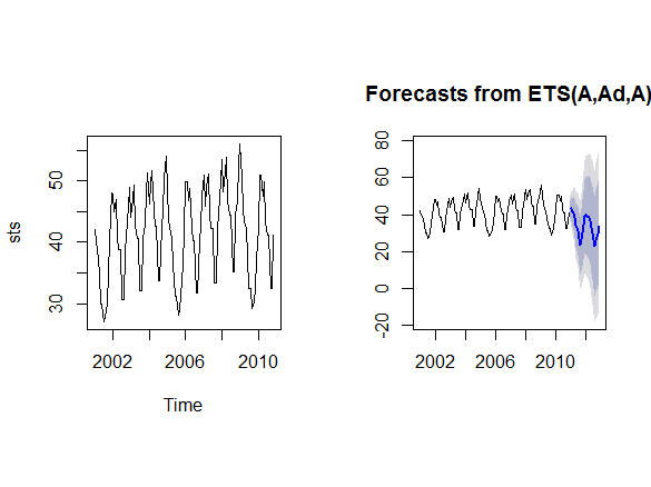
 plot(sts)
 
 #par(mfrow = c(2, 2))  

 # Forecast using ETS method 
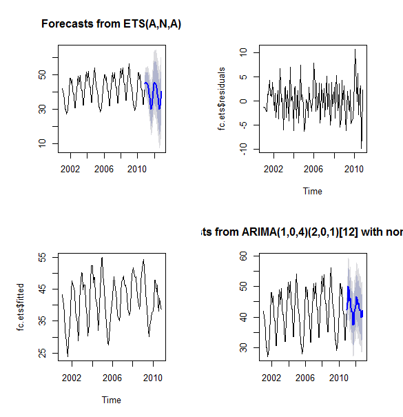
 fc.ets = forecast(sts)
 plot(fc.ets)
 plot(fc.ets$residuals)
 plot(fc.ets$fitted)


 # Forecast using ARIMA method
 ar = auto.arima(sts)
 ar
 fc.arima = forecast(ar)
 fc.arima
 plot(fc.arima)

 accuracy(fc.ets)
 accuracy(fc.arima)

Exponential Smoothing

Names

• AKA: exponentially weighted moving average (EWMA)
• Equivalent to ARIMA (0,1,1) model with no constant term

Used for

• smoothed data for presentation
• make forecasts
• simple moving average: past observations are weighted equally
• exponential smoothing: assigns exponentially decreasing weights over time

Formula

{x_t} - raw data sequence

{s_t} - output of the exponential smoothing algorithm (estimate of the next value of x)

α - smoothing factor, 0 < α < 1.

${\begin{aligned}s_{1}&=x_{0}\\s_{t}&=\alpha x_{t-1}+(1-\alpha )s_{t-1},t>1\end{aligned}}$

Choosing right α

• no formal way of choosing α
• statistical technique may be used to optimize the value of α (e.g. OLS)
• the bigger the α the close it gets to naive forecasting (the same ports as original series with one period lag)

Double Exponential Smoothing

• Simple exponential smoothing does not do well when there is a trend (there will be always bias)
• Double exponential smoothing is a group of methods dealing with the problem

Holt-Winters double exponential smoothing

Input

• {x_t} - raw data sequence of observations
• t = 0

Model

• {s_t} - smoothed value for time t
• {b_t} - best estimate of the trend at time t

${\begin{aligned}s_{1}&=x_{0}\\b_{1}&=x_{1}-x_{0}\\\end{aligned}}$

And for t > 1 by

${\begin{aligned}s_{t}&=\alpha x_{t}+(1-\alpha )(s_{t-1}+b_{t-1})\\b_{t}&=\beta (s_{t}-s_{t-1})+(1-\beta )b_{t-1}\\\end{aligned}}$

where α is the data smoothing factor, 0 < α < 1, and β is the trend smoothing factor, 0 < β < 1.

Output

• F_t+m - an estimate of the value of x at time t+m, m>0 based on the raw data up to time t

To forecast beyond x_t

${\begin{aligned}F_{t+m}&=s_{t}+mb_{t}\end{aligned}}$

Triple exponential smoothing

• takes into account seasonal changes as well as trends
• first suggested by Holt's student, Peter Winters, in 1960

Input

• {x_t} - raw data sequence of observations
• t = 0
• L length a cycle of seasonal change

The method calculates:

• a trend line for the data
• seasonal indices that weight the values in the trend line based on where that time point falls in the cycle of length L.

• {s_t} represents the smoothed value of the constant part for time t.
• {b_t} represents the sequence of best estimates of the linear trend that are superimposed on the seasonal changes
• {c_t} is the sequence of seasonal correction factors
• c_t is the expected proportion of the predicted trend at any time t mod L in the cycle that the observations take on
• To initialize the seasonal indices c_t-L there must be at least one complete cycle in the data

The output of the algorithm is again written as F_t+m, an estimate of the value of x at time t+m, m>0 based on the raw data up to time t. Triple exponential smoothing is given by the formulas

${\begin{aligned}s_{0}&=x_{0}\\s_{t}&=\alpha {\frac {x_{t}}{c_{t-L}}}+(1-\alpha )(s_{t-1}+b_{t-1})\\b_{t}&=\beta (s_{t}-s_{t-1})+(1-\beta )b_{t-1}\\c_{t}&=\gamma {\frac {x_{t}}{s_{t}}}+(1-\gamma )c_{t-L}\\F_{t+m}&=(s_{t}+mb_{t})c_{t-L+((m-1){\pmod {L}})},\end{aligned}}$

where α is the data smoothing factor, 0 < α < 1, β is the trend smoothing factor, 0 < β < 1, and γ is the seasonal change smoothing factor, 0 < γ < 1.

The general formula for the initial trend estimate b₀ is:

${\begin{aligned}b_{0}&={\frac {1}{L}}({\frac {x_{L+1}-x_{1}}{L}}+{\frac {x_{L+2}-x_{2}}{L}}+\ldots +{\frac {x_{L+L}-x_{L}}{L}})\end{aligned}}$

Setting the initial estimates for the seasonal indices c_i for i = 1,2,...,L is a bit more involved. If N is the number of complete cycles present in your data, then:

${\begin{aligned}\\c_{i}&={\frac {1}{N}}\sum _{j=1}^{N}{\frac {x_{L(j-1)+i}}{A_{j}}}\quad \forall i&=1,2,\ldots ,L\\\end{aligned}}$

where

${\begin{aligned}A_{j}&={\frac {\sum _{i=1}^{L}x_{L(j-1)+i}}{L}}\quad \forall j&=1,2,\ldots ,N\end{aligned}}$

Note that A_j is the average value of x in the jth cycle of your data.

ETS

• Error, Trend, Seasonality

Overriding parameters

rawdata <- read.table("http://training-course-material.com/images/1/19/Sales-time-series.txt",h=T)
rawdata$Date <- as.Date(rawdata$Date)
head(rawdata)
plot(rawdata)

# Using build in ts object
sts <- ts(rawdata$Sales,start=2001,frequency=12)
plot(sts)

# Forecast using ETS method
model.ets = ets(sts,model="ANA")
fc.ets = forecast(model.ets)

model.ets1 = ets(sts,model="AAA",beta=0.2)
fc.ets1 = forecast(model.ets1)
plot(fc.ets1)

accuracy(fc.ets)
accuracy(fc.ets1)

See Also

• http://www.jstatsoft.org/v27/i03/paper
• http://robjhyndman.com/talks/MelbourneRUG.pdf