Prediction

title

Regresssion

author

Yolande Tra

Introduction to Simple Linear Regression。

Simple Regression

In simple linear regression, we predict scores on one variable from the scores on a second variable.

• Criterion variable: The variable we are predicting, referred to as Y.
• Predictor variable: The variable we are basing our predictions on, referred to as X.

When there is only one predictor variable, the prediction method is called simple regression

• In simple linear regression, the predictions of Y when plotted as a function of X form a straight line.

Simple Regression Example。

Data in the table are plotted in the graph below.

• there is a positive relationship between X and Y.
• If you were going to predict Y from X,
• the higher the value of X, the higher your prediction of Y.

	X	Y
	1.00	1.00
	2.00	2.00
	3.00	1.30
	4.00	3.75
	5.00	2.25

Linear regression。

• Linear regression consists of finding the best-fitting straight line through the points.
• The best-fitting line is called a regression line

Example

The black diagonal line is the regression line and consists of the predicted score on Y for each possible value of X. The vertical lines from the points to the regression line represent the errors of prediction. the red point is very near the regression line; its error of prediction is small. By contrast, the yellow point is much higher than the regression line and therefore its error of prediction is large.

Regression Line。

The error of prediction

The error of prediction for a point is the value of the point minus the predicted value (the value on the line)

Example

• the predicted values (Y') and the errors of prediction (Y-Y').
• the first point has a Y of 1.00 and a predicted Y of 1.21. Therefore its error of prediction is -0.21.

X	Y	Y'	Y-Y'	(Y-Y')2
1.00	1.00	1.210	-0.210	0.044
2.00	2.00	1.635	0.365	0.133
3.00	1.30	2.060	-0.760	0.578
4.00	3.75	2.485	1.265	1.600
5.00	2.25	2.910	-0.660	0.436

Regression Line。

The Best Fitting Line

What does it meant by "best fitting line" ?

• By far the most commonly used criterion for the best fitting line is the line that minimizes the sum of the squared errors of prediction.
• That is the criterion that was used to find the line in previous regression line graph.
• The last column in the previous table shows the squared errors of prediction.
• The sum of the squared errors of prediction shown in the previous table is lower than it would be for any other regression line.

The Formula for a Regression Line。

The formula for a regression line

Y' = bX + A
where Y' is the predicted score, b is the slope of the line, and A is the Y intercept. 

Example

The equation for the line in the previous graph is

Y' = 0.425X + 0.785

• For X = 1, Y' = (0.425)(1) + 0.785 = 1.21
• For X = 2, Y' = (0.425)(2) + 0.785 = 1.64

Computing the Regression Line。

• In the age of computers, the regression line is typically computed with statistical software.
• However, the calculations are relatively easy are given here for anyone who is interested.

The calculations are based on the statistics below.

M_X is the mean of X

M_Y is the mean of Y

s_X is the standard deviation of X

s_Y is the standard deviation of Y

r is the correlation between X and Y

MX	MY	sX	sY	r
3	2.06	1.581	1.072	0.627

The Slope of the Regression Line。

The slope (b) can be calculated as follows:

b = r sY/sX

and the intercept (A) can be calculated as

A = MY - bMX
 

For these data,

b = (0.627)(1.072)/1.581 = 0.425
A = 2.06 - (0.425)(3)=0.785

• The calculations have all been shown in terms of sample statistics rather than population parameters.
• The formulas are the same; simply use the parameter values for means, standard deviations, and the correlation.

Standardized Variables。

• The regression equation is simpler if variables are standardized so that their means are equal to 0 and standard deviations are equal to 1, for then b = r and A = 0.
• This makes the regression line:

ZY' = (r)(ZX)
where ZY' is the predicted standard score for Y, r is the correlation, and ZX is the standardized score for X. 

Note that the slope of the regression equation for standardized variables is r.

Example。

The case study, Predicting GPA contains high school and university grades for 105 computer science majors at a local state school.

• We now consider how we could predict a student's university GPA if we knew his or her high school GPA.
• The correlation is 0.78 The regression equation is

GPA' = (0.675)(High School GPA) + 1.097

• A student with a high school GPA of 3 would be predicted to have a university GPA of

GPA' = (0.675)(3) + 1.097 = 3.12
 

• The graph shows University GPA as a function of High School GPA
• There is a strong positive relationship between them

Assumptions。

• It may surprise you, but the calculations shown in this section are assumption free.
• Of course, if the relationship between X and Y is not linear, a different shaped function could fit the data better.
• Inferential statistics in regression are based on several assumptions.

Quiz。

1 The formula for a regression equation is

What would be the predicted Y score for a person scoring 4 on X?

Answer >>

10

Plug X equals 4 into the equation to find Y'equals to 3(4) - 2 is 10

2 Suppose it is possible to predict a person's score on Test B from the person's score on Test A. The regression equation is:

Quiz。

What is a person's predicted score on Test B assuming this person got a 40 on Test A?

Answer >>

101.5

Plug A equals to 40 into the equation to find B'equals to 2.3(40) + 9.5 is 101.5

3 Suppose a person got a score of 32.5 on Test A and a score of 95.25 on Test B. Using the same regression equation as in the previous problem,

what is the error of prediction for this person?

Answer >>

11

Predicted value, B' equals to 2.3(32.5) + 9.5 is 84.25; Error of prediction is B - B' equals to 95.25 - 84.25 equals to 11

4 What is the most common criterion used to determine the best-fitting line?

	The line that goes through the most points
	The line that has the same number of points above it as below it
	The line that minimizes the sum of squared errors of prediction

5

Answer >>

The line that minimizes the sum of squared errors of prediction

The most common criterion used to determine the best-fitting line is the line that minimizes the sum of squared errors of prediction. This line does not need to go through any of the actual data points, and it can have a different number of points above it and below it.

	True
	False

6

Answer >>

The line that minimizes the sum of squared errors of prediction

Someone who scored the mean on X would be predicted to score the mean on Y.

	0.00
	0.25
	0.50
	0.10

Answer >>

0.25

b is r(sY/sX). 0.5^0.5 equals to .25

Partitioning Sums of Squares。

One useful aspect of regression is that it can divide the variation in Y into two parts:

• the variation of the predicted scores
• the variation in the errors of prediction

The variation of Y

• the sum of squares Y
• defined as the sum of the squared deviations of Y from the mean of Y

Formula of the Variation of Y。

In the population, the formula of The variation of Y

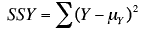where SSY is the sum of squares Y and 
Y is an individual value of Y, and my is the mean of Y

Example。

The mean of Y is 2.06 and SSY is the sum of the values in third column and is equal to 4.597

When computed in a sample, you should use the sample mean, M, in place of the population mean.

Example。

• The column Y' were computed according to this equation.
• The column y' contains deviations of Y' from the mean Y'
• The column y'² is the square of this column.
• The column Y-Y' contains the actual scores (Y) minus the predicted scores (Y')
• The column (Y-Y')² contains the squares of these errors of prediction

Sum of the squared deviations from the mean 。

SSY is the sum of the squared deviations from the mean.

• It is therefore the sum of the y2 column and is equal to 4.597.
• SSY can be partitioned into two parts:

1. the sum of squares predicted (SSY')

• The sum of squares predicted is the sum of the squared deviations of the predicted scores from the mean predicted score.
• In other words, it is the sum of the y'2 column and is equal to 1.806

2.the sum of squares error (SSE)

• The sum of squares error is the sum of the squared errors of prediction.
• It is there fore the sum of the (Y-Y')² column and is equal to 2.791.
• This can be summed up as:

SSY = SSY' + SSE 
4.597 = 1.806 + 2.791

Example。

The sum of y and the sum of y' are both zero

This will always be the case because these variables were created by subtracting their respective means from each value.

The mean of Y-Y' is 0

This indicates that although some Y's are higher than there respective Y's and some are lower, the average difference is zero.

SSY is the total variation
SSY' is the variation explained
SSE is the variation unexplained

Therefore, the proportion of variation explained can be computed as:

Proportion explained = SSY'/SSY

Similarly, the proportion not explained is:

Proportion not explained = SSE/SSY

r²。

There is an important relationship between the proportion of variation explained and Pearson's correlation:

r² is the proportion of variation explained

Therefore,

• if r = 1, then the proportion of variation explained is 1
• if r = 0, then the proportion explained is 0;
• if r = 0.4, then the proportion of variation explained is 0.16

Since the variance is computed by dividing the variation by N (for a population) or N-1 (for a sample), the relationships spelled out above in terms of variation also hold for variance

Example

• the first term is the variance total
• the second term is the variance of Y'
• the last term is the variance of the errors of prediction (Y-Y')

Similarly, r2 is the proportion of variance explained as well as the proportion of variation explained.

Summary Table。

It is often convenient to summarize the partitioning of the data in a table.

• The degrees of freedom column (df) shows the degrees of freedom for each source of variation.
• The degrees of freedom for the sum of squares explained is equal to the number of predictor variables.
• This will always be 1 in simple regression.
• The error degrees of freedom is equal to the total number of observations minus 2.
• In this example, it is 5 - 2 = 3.
• The total degrees of freedom is the total number of observations minus 1.

Source	Sum of Squares	df	Mean Square
Explained	1.806	1	1.806
Error	2.791	3	0.930
Total	4.597	4

</>

Quiz

1 If these data are converted to deviation scores, the last value (15) would have a value of

Y
 2
 9
11
13
15

Answer >>

15

To compute a deviation score you subtract the mean. 15 - 10 is 5.

2 Compute the sum of squares Y.

Y
 2
 9
11
13
15

Answer >>

100

To compute SSY, first compute the deviation scores (y) by subtracting the mean (10) from each number. Then square these values and add them together: (-8)2 + (-1)2 + 12 + 32 + 52 equals to 100

3 If SSY is 25.5 and SSY' is 18.3, what is SSE?

Y
 2
 9
11
13
15

Answer >>

7.2

SSY is SSY' + SSE; SSE is SSY - SSY' 25.5 - 18.3 equals to 7.2

4 The larger ________ is, the larger the proportion of variation explained is.

	SSY
	SSY'
	SSE
	Y

Answer >>

False

Proportion of variation explained is SSY'/SSY, so as SSY' increases, so does the proportion of variation explained.

5 The proportion of variation explained is 0.3. If SSY is 20, what is SSY'?

Answer >>

6

Proportion explained is SSY'/SSY; SSY' is (.3)(20) equals to 6

6 If r is .84, what proportion of variation is explained?

Answer >>

0.71

r² is the proportion of variation explained. (.84)2 is .71

The standard error of the estimate。

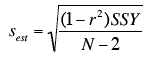
The standard error of the estimate

• is closely related to this quantity and is defined below:
• is a measure of the accuracy of predictions

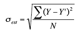sest is the standard error of the estimate,
Y        - actual score
Y'       - predicted score
Y-Y'     - differences between the actual scores and the predicted scores.
Σ(Y-Y')2 - SSE 
N        - number of pairs of scores

Simple Example

• The graphs below shows two regression examples.
• You can see that in graph A, the points are closer to the line then they are in graph B.
• Therefore, the predictions in Graph A are more accurate than in Graph B.

Example。

Assume the data below are the data from a population of five X-Y pairs

• The last column shows that the sum of the squared errors of prediction is 2.791.
• Therefore, the standard error of the estimate is:

Formula for the Standard Error

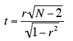
There is a version of the formula for the standard error in terms of Pearson's correlation:

where ρ is the population value of Pearson's correlation

SSY is

Similar formulas are used when the standard error of the estimate is computed from a sample rather than a population.

• The only difference is that the denominator is N-2 rather than N, since two parameters (the slope and the intercept) were estimated in order to estimate the sum of squares
• Formulas comparable to the ones for the population are shown below.

Example。

For the example data,

• μ_y = 2.06
• SSY = 4.597
• ρ= 0.6268.

Therefore,

which is the same value computed previously. </>

Quiz

1 In a regression line, the ________ the standard error of the estimate is, the more accurate the predictions are.

	larger
	smaller
	The standard error of the estimate is not related to the accuracy of the predictions.

Answer >>

smaller

The standard error of the estimate is a measure of the accuracy of predictions. The regression line is the line that minimizes the sum of squared deviations of prediction (also called the sum of squares error), and the standard error of the estimate is the square root of the average squared deviation.

2 Linear regression was used to predict Y from X in a certain population. In this population, SSY is 50, the correlation between X and Y is .5, and N is 100. What is the standard error of the estimate?

Answer >>

0.61

The standard error of the estimate for a population is sqrt[(1-rho2)*SSY/N]

sqrt[(1-.52)*50/100] equals .61

3 You sample 10 people in a high school to try to predict GPA in 10th grade from GPA in 9th grade. You determine that SSE = 5.8. What is the standard error of the estimate?

Answer >>

0.85

The standard error of the estimate for a sample is sqrt[SSE/(N-2)]

sqrt[5.8/8] equals to .85

4 The graph below represents a regression line predicting Y from X. This graph shows the error of prediction for each of the actual Y values. Use this information to compute the standard error of the estimate in this sample.

Answer >>

1

The standard error of the estimate for a sample is sqrt[SSE/(N-2)].

SSE is the sum of the squared errors of prediction,

so SSE is (-.2)2 + (.4)2 + (-.8)2 + (1.3)2 + (-.7)2 equals to 3.02;

sqrt(3.02/3) is 1.0

Inferential Statistics for b and r。

Assumptions

• Although no assumptions were needed to determine the best-fitting straight line, assumptions are made in the calculation of inferential statistics.
• Naturally, these assumptions refer to the population, not the sample.

1. Linearity: The relationship between the two variables is linear.
2. Homoscedasticity: The variance around the regression line is the same for all values of X. A clear violation of this assumption is shown in below. (Notice that the predictions for students with high high-school GPAs are very good, whereas the predictions for students with low high-school GPAs are not very good. In other words, the points for students with high high-school GPAs are close to the regression line, whereas the points for low high-school GPA students are not.)
3. The errors of prediction are distributed normally. This means that the deviations from the regression line are normally distributed. It does not mean that X or Y is normally distributed.

Significance Test for the Slope (b)

The general formula for a t test

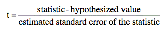
As applied here, the statistic is the sample value of the slope (b) and the hypothesized value is 0.

The number of degrees of freedom for this test is

df = N-2
where N is the number of pairs of scores.

The estimated standard error of b is computed using the following formula

sb is the estimated standard error of b, 
sest is the standard error of the estimate
SSX is the sum of squared deviations of X from the mean of X

SSX is calculated as

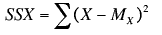where Mx is the mean of X

The standard error of the estimate can be calculated as

Example。

• The column X has the values of the predictor variable
• The column Y has the values of the criterion variable
• The column x has the differences between the values of column X and the mean of X
• The column x² is the square of the x column
• The column y has the differences between the values of column Y and the mean of Y.
• The column y² is simply square of the y column

The standard error of the estimate

The computation of the standard error of the estimate (s_est) for these data is shown in the section on the standard error of the estimate. It is equal to 0.964.

sest = 0.964

SSX

SSX is the sum of squared deviations from the mean of X. i.e. it is equal to the sum of the x2 column and is equal to 10.

SSX = 10.00

We now have all the information to compute the standard error of b:

the slope (b) is

b= 0.425. 
df = N-2 = 5-2 = 3.

• The p value for a two-tailed t test is 0.26.
• Therefore, the slope is not significantly different from 0.

Confidence Interval for the Slope。

• The method for computing a confidence interval for the population slope is very similar to methods for computing other confidence intervals.
• For the 95% confidence interval, the formula is:

lower limit: b - (t.95)(sb)
upper limit: b + (t.95)(sb)
where t.95 is the value of t to use for the 95% confidence interval

Example。

• The values of t to be used in a confidence interval can be looked up in a table of the t distribution.
• A small version of such a table is shown above.
• The first column, df, stands for degrees of freedom.
• You can also use the "inverse t distribution" calculator to find the t values to use in a confidence interval.
• Applying these formulas to the example data,

lower limit: 0.425 - (3.182)(0.305) = -0.55
upper limit: 0.425 + (3.182)(0.305) = 1.40

Significance Test for the Correlation。

The formula for a significance test of Pearson's correlation is shown below:

where N is the number of pairs of scores. 

For the example data,

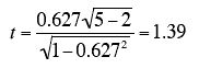
Notice that this is the same t value obtained in the t test of b. As in that test, the degrees of freedom is

N - 2 = 5 -2 = 3.

Quiz

1 Which of the following are assumptions made in the calculation of regression inferential statistics?

	A:The errors of prediction are normally distributed.
	B:X is normally distributed.
	C:Y is normally distributed.
	D:The variance around the regression line is the same for all values of X.
	E:The relationship between X and Y is linear.

Answer >>

A,D,E

The assumptions are linearity, homoscedasticity, and normally distributed errors. See the text for more information.

2 The slope of a regression line is 0.8, and the standard error of the slope is 0.3. The sample used to compute this regression line consisted of 12 participants. Compute the 95% confidence interval for the slope. Type the upper limit of the confidence interval in the box below.

Answer >>

1.47

Use the table in this section or the inverse t distribution calculator to find that the critical value is t(N-2).

t(10) s 2.23.

The upper limit of the 95% CI is b + (t)(sb)

.8 + 2.23(.3) equals to 1.47.

3 In a sample of 20, the correlation between two variables is .5. Determine if this correlation is significant at the .05 level by calculating the t value.

Answer >>

2.45

t is (r) sqrt(N-2)/sqrt(1-r2) equals to (0.5) sqrt(18)/sqrt(1-.25) is 2.45 (This is significant at the .05 level.)

4 Calculate the lower limit of the 95% confidence interval for the correlation of .75 (N = 25).

Answer >>

0.505

First, convert r to z' (so .75 -> .973). The standard error of z' is 1/sqrt(N-3)is .213.

Lower limit of CI is .973 - 1.96(.213) equals to 0.556. Now convert back from z' to r. r is .505