Differences between Two Means (Independent Groups)

Learning Objectives

State the assumptions for testing the difference between two means
Estimate the population variance assuming homogeneity of variance
Compute the standard error of the difference between means
Compute t and p for the difference between means.

Differences between Two Means (Independent Groups)

It is more common to test the difference between means than in the specific values of the means themselves
We assume that the means we test come from independent groups, i.e. two separate groups of subjects
Later we will test for differences between the means of two conditions in designs where only one group of subjects is used and each subject is tested in each condition.

Animal Research Example

Students rated (on a 7-point scale) whether they thought animal research is wrong
The sample sizes, means, and variances are shown separately for males and females in the table below

Means and Variances in Animal Research study
Condition	n	Mean	Variance
Females	17	5.353	2.743
Males	17	3.882	2.985

The females rated animal research as more wrong than did the males
This sample difference between the female mean of 5.35 and the male mean of 3.88 is 1.47
Is there a difference in the population means?

Testing Means Assumptions

The two populations have the same variance (homogeneity of variance)
The populations are normally distributed
Each value is sampled independently from each other value, ie. each subject provide only one value

If a subject provides two scores, then the scores are not independent. (see the section on the correlated t test)
Small-to-moderate violations of assumptions 1 and 2 do not make much difference (simulation in the next section)
It is important not to violate assumption 3!

Calculating t

We saw the following general formula for significance testing in the section on testing a single mean:

The statistic is the difference between sample means and our hypothesized value is 0
The hypothesized value is the null hypothesis that the difference between population means is 0

Now we will compute a significance test on the difference between the mean score of the males and the mean score of the females.
For this calculation, we will make the three assumptions specified above.
The first step is to compute the statistic, which is simply the difference between means.

M1 - M2 = 5.3523 - 3.8824 = 1.470

Since the hypothesized value is 0, we do not need to subtract it from the statistic

The next step is to compute the estimate of the standard error of the statistic. In this case, the statistic is the difference between means so the estimated standard error of the statistic is ().

Calculating standard error

The formula for the standard error of the difference in means in the population is (see sampling distributions):

In order to estimate SE, we estimate σ² and use that estimate in place of σ²

Calculating Mean Squared Error (MSE)

Since we are assuming the population variances are the same, we estimate this variance by averaging our two sample variances. Thus, our estimate of variance is computed using the following formula:

where MSE is our estimate of σ². In this example,

MSE = (2.743 + 2.985)/2 = 2.864

Since n (the number of scores in each condition) is 17,

 =  =  = = 0.5805

The next step is to compute t by plugging these values into the formula:

t = 1.47/.5805 = 2.533

Interpreting the results

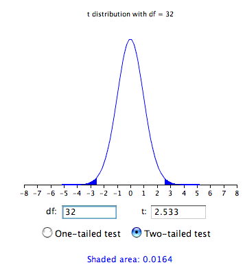
What is the probability of getting a t as large or larger than 2.53 or as small or smaller than -2.53
The degrees of freedom is the number of independent estimates of variance on which MSE is based

 df = (n1 - 1) + (n2 -1) 
 16 + 16 = 32.

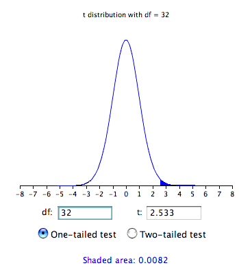
Figure below shows that the probability value for a two-tailed test is 0.0164
The two-tailed test is used when the null hypothesis can be rejected regardless of the direction of the effect.

Computations for Unequal Sample Sizes (optional)

The calculations are somewhat more complicated when the sample sizes are not equal
One consideration is that MSE, the estimate of variance, counts the sample with the larger sample size more than the sample with the smaller sample size
Computationally this is done by computing the sum of squares error (SSE) as follows:


 M1 is the mean for group 1
 M2 is the mean for group 2

Consider the following small example:

Unequal n
Group 1	Group 2
3	2
4	4
5

M1 = 4 and M2 = 3.

SSE = (3-4)² + (4-4)² + (5-4)² + (2-3)² + (4-3)² = 4

Then, MSE is computed by:

MSE = SSE/df
where the degrees of freedom (df) are computed as before: 

df = (n1 -1) + (n2 -1) = (3-1) + (2-1) = 3.

MSE = SSE/df = 4/3 = 1.333.

The formula

 is replaced by

where nh is the harmonic mean of the sample sizes and is computed as follows:

nh =    = 2.4.

and,

 =  = 1.054.

Therefore,

t = (4-3)/1.054 = 0.949

and the two-tailed p = 0.413.

Questions

	the null hypothesis.
	the mean of all numbers.
	the difference between sample means.
	the significance level.

Differences between Two Means (Independent Groups)

Contents

Learning Objectives