R - Multiple regression
Covered Materials
- assumptions of multiple regression
- regression equation
- regression coefficient (weights)
- beta weight
- R and r
- partial slope
- sum of squares explained in a multiple regression compared to sum of squares in simple regression
- R2 and proportion explained
- R2 significance test
- Complete and reduced model for significance
Assumptions
- No assumptions are necessary for:
- computing the regression coefficients
- partitioning the sum of squares
- Interpreting inferential statistics makes 3 major assumptions
- Moderate violations of the assumptions do not pose a serious problem for testing the significance of predictor variables
- Even small violations of these assumptions pose problems for confidence intervals on predictions for specific observations
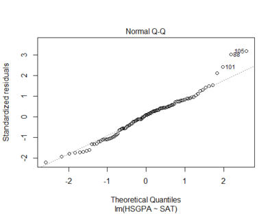
Residuals are normally distributed
- residuals are the errors of prediction (differences between the actual and the predicted scores)
- Q-Q plot is usually to test residual normality
qqnorm(m$residuals)
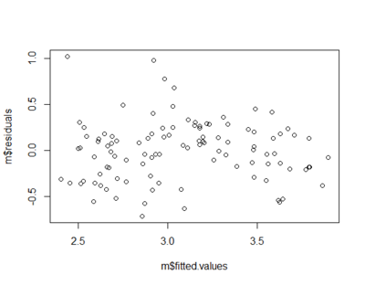
Homoscedasticity
- variances of the errors of prediction are the same for all predicted values
 plot(m$fitted.values,m$residuals)
 # see also plot(m)
- In the picture below the errors of prediction are much larger for observations with low-to-medium predicted scores than for observations with high predicted scores
- Confidence interval on a low predicted UGPA would underestimate the uncertainty
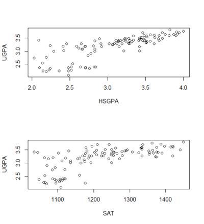
Linearity
- relationship between each predictor and the criterion variable is linear
- If this assumption is not met, then the predictions may systematically overestimate the actual values for one range of values on a predictor variable and underestimate them for another.
- if it is know that the variables are not linear, a transformation can be use to the linear form
plot(UGPA ~ HSGPA)
plot(UGPA ~ SAT)
Data Used
File:MultipleRegression-GPA.txt
rawdata <- read.table("http://training-course-material.com/images/4/4b/MultipleRegression-GPA.txt",h=T)
head(rawdata)

# Just nameing them more convinently
HSGPA <- rawdata$high_GPA
SAT <- rawdata$math_SAT + rawdata$verb_SAT
UGPA <- rawdata$univ_GPA
Building Model
m <- lm(UGPA ~ HSGPA + SAT)
lm(formula = UGPA ~ HSGPA + SAT)

Coefficients:
(Intercept)        HSGPA          SAT
  0.5397848    0.5414534    0.0007918
Validating Model
summary(m)
Call:
lm(formula = UGPA ~ HSGPA + SAT)

Residuals:
     Min       1Q   Median       3Q      Max
-0.68072 -0.13667  0.01137  0.17012  0.92983

Coefficients:
             Estimate Std. Error t value Pr(>|t|)
(Intercept) 0.5397848  0.3177784   1.699   0.0924 .
HSGPA       0.5414534  0.0837479   6.465 3.53e-09 ***
SAT         0.0007918  0.0003868   2.047   0.0432 *
---
Signif. codes:  0 ‘***’ 0.001 ‘**’ 0.01 ‘*’ 0.05 ‘.’ 0.1 ‘ ’ 1

Residual standard error: 0.2772 on 102 degrees of freedom
Multiple R-squared: 0.6232,	Adjusted R-squared: 0.6158
F-statistic: 84.35 on 2 and 102 DF,  p-value: < 2.2e-16
Interpreting the results
Regression is express my the formula:
UGPA = b1*HSGPA + b2*SAT + A
- b1 and b2 are regression coefficients
- a regression coefficient is the slope of the linear relationship between:
- the criterion variable and
- the part of a predictor variable that is independent of all other predictor variables
Example
- the regression coefficient for HSGPA can be computed by:
- first predicting HSGPA from SAT
m.HSGPA.SAT = lm(HSGPA ~ SAT)
Call:
lm(formula = HSGPA ~ SAT)

Coefficients:
(Intercept)          SAT
  -1.313853     0.003594
- calculating the errors of prediction (m.HSGPA.SAT$residuals)
- find the slope of the UGPA ~ m.HSGPA.SAT$residuals
lm(UGPA ~ m.HSGPA.SAT$residuals)
Call:
lm(formula = UGPA ~ m.HSGPA.SAT$residuals)

Coefficients:
          (Intercept)  m.HSGPA.SAT$residuals
               3.1729                 0.5415
The 0.5415 is the same value as b1
Further coefficient interpretations
The regression coefficient for HSGPA (b1) is the slope of the relationship between the criterion variable (UGPA) and the part of HSGPA that is independent of (uncorrelated with) the other predictor variables (SAT in this case).
It represents the change in the criterion variable associated with a change of one in the predictor variable when all other predictor variables are held constant.
Since the regression coefficient for HSGPA is 0.54, this means that, holding SAT constant, a change of one in HSGPA is associated with a change of 0.54 in UGPA'.
Partial Slope
The slope of the relationship between the part of a predictor variable independent of other predictor variables and the criterion is its partial slope
Thus the regression coefficient of 0.541 for HSGPA and the regression coefficient of 0.008 for SAT are partial slopes.
Each partial slope represents the relationship between the predictor variable and the criterion holding constant all of the other predictor variables.
Beta Weight
- It is difficult to compare the coefficients for different variables directly because they are measured on different scales
- A difference of 1 in HSGPA is a fairly large difference (0.54), whereas a difference of 1 on the SAT is negligible (0.008).
- standardization of the variables to standard deviation of 1 solves the problem
- A regression weight for standardized variables is called a beta weight (designated as β)
 install.packages("yhat")
 library("yhat")

 r <- regr(m)
 r$Beta
- For these data, the beta weights are 0.625 and 0.198
- These values represent the change in the criterion (in standard deviations) associated with a change of one standard deviation on a predictor [holding constant the value(s) on the other predictor(s)]
- Clearly, a change of one standard deviation on HSGPA is associated with a larger difference than a change of one standard deviation of SAT
- In practical terms, this means that if you know a student's HSGPA, knowing the student's SAT does not aid the prediction of UGPA much
- However, if you do not know the student's HSGPA, his or her SAT can aid in the prediction since the β weight in the simple regression predicting UGPA from SAT is 0.68
 m1 <- lm(UGPA ~ SAT)
 regr(m1)$Beta_Weights
- the β weight in the simple regression predicting UGPA from HSGPA is 0.78
 m1 <- lm(UGPA ~ HSGPA)
 regr(m1)$Beta_Weights
- As is typically the case, the partial slopes are smaller than the slopes in simple regression.
Sum of Squares
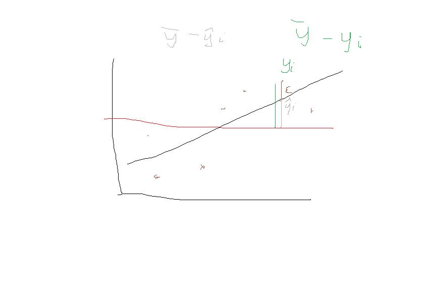
Total sum of squares (TSS or SSY)
- Sum of the squared difference between the actual Y and the mean of Y
- ith data point
- the estimate of the mean
- tells us how much variation there is in the dependent variable
sum((UGPA - mean(UGPA))^2)
Explained sum of squares (ESS or SSY')
- Sum of the squared differences between the predicted Y and the mean of Y,
- = Yhat
- ESS tells us how much of the variation in the dependent variable our model explained
sum((m$fitted.values - mean(UGPA))^2)
Residual sum of squares (RSS or SSE)
- Sum of the squared differences between the actual Y and the predicted Y
- it is how much of the variation in the dependent variable our model did not explain
sum((UGPA - m$fitted.values)^2)
Calculating sum of squares in R
 TSS = sum((UGPA - mean(UGPA))^2)
 ESS = sum((m$fitted.values - mean(UGPA))^2)
 RSS = sum((UGPA - m$fitted.values)^2)
 # TODO: add aov function method
> TSS
[1] 20.79814
> ESS
[1] 12.96135
> RSS
[1] 7.836789
Multiple Correlation and Proportion Explained
Proportion Explained = SSY'/SSY = R2
ProportionExplained = ESS/TSS
ProportionExplained
[1] 0.6231977
 m <- lm(UGPA ~ HSGPA + SAT)
 summary(m)
Call:
lm(formula = UGPA ~ HSGPA + SAT)

Residuals:
     Min       1Q   Median       3Q      Max
-0.68072 -0.13667  0.01137  0.17012  0.92983

Coefficients:
             Estimate Std. Error t value Pr(>|t|)
(Intercept) 0.5397848  0.3177784   1.699   0.0924 .
HSGPA       0.5414534  0.0837479   6.465 3.53e-09 ***
SAT         0.0007918  0.0003868   2.047   0.0432 *
---
Signif. codes:  0 ‘***’ 0.001 ‘**’ 0.01 ‘*’ 0.05 ‘.’ 0.1 ‘ ’ 1

Residual standard error: 0.2772 on 102 degrees of freedom
Multiple R-squared: 0.6232,	Adjusted R-squared: 0.6158
F-statistic: 84.35 on 2 and 102 DF,  p-value: < 2.2e-16
Confounding
- the sum of squares explained (ESS) for these data is 12.96
- How is this value divided between HSGPA and SAT?
- it is not the same as prediction of UGPA in separate simple regressions for HSGPA and SAT
Predictors	Sum of Squares
HSGPA	        12.64 (simple regression)
SAT	        9.75  (simple regression)
HSGPA and SAT	12.96 (multiple regression)
 m <- lm(UGPA ~ HSGPA + SAT)
 ESS = sum((m$fitted.values - mean(UGPA))^2)
 # SAT has bee left out
 m.hsgpa <- lm(UGPA ~  HSGPA)
 ess.hsgpa <- sum((m.hsgpa$fitted.values - mean(UGPA))^2)
 # HSGPA has been left out
 m.sat <- lm(UGPA ~  SAT)
 ess.sat <- sum((m.sat$fitted.values - mean(UGPA))^2)
 ess.hsgpa # 12.63942
 ess.sat   # 9.749823
- If the sum of ESS in simple regressions is higher than the ESS in multiple regression, it means the predictors are correlated (r = .78)
- Much of the variance in UGPA is confounded between HSGPA and SAT
- The variance in UGPA could be explained by either HSGPA or SAT
- is counted twice if the sums of squares for HSGPA and SAT are simply added.
Proportion of variable explained
Source	                       SS   Proportion
HSGPA (unique)	             3.21   0.15
SAT (unique)	             0.32   0.02
HSGPA and SAT (Confounded)   9.43   0.45
Error	                     7.84   0.38
Total	                    20.80  1.00
 HSGPA.UNIQUE <- ESS - ess.sat
 HSGPA.UNIQUE # 3.211531
 SAT.UNIQUE   <- ESS - ess.hsgpa
 SAT.UNIQUE    # 0.3219346
 HSGPA.SAT.Confounded = ESS - (HSGPA.UNIQUE + SAT.UNIQUE)
 HSGPA.SAT.Confounded # 9.427889


