Central Tendency
What is Central Tendency?
|
Student | Dataset A | Dataset B | Dataset C |
|---|---|---|---|---|
| You | 3 | 3 | 3 | |
| Sara's | 3 | 4 | 2 | |
| Jake's | 3 | 4 | 2 | |
| Maria's | 3 | 4 | 2 | |
| Tom's | 3 | 4 | 2 |
- Three possible outcomes of the 5-point make-up quiz are shown in Table above.
- Which of the three datasets would make you happiest?
- Dataset A: Your score is at the exact center of the distribution.
- Dataset B: Your score is below the center of the distribution.
- Dataset C: Your score is above the center of the distribution.
Definitions of Center
There are three different ways of defining the center of a distribution.
Balance Scale
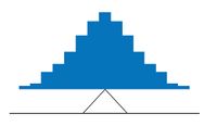
- One definition of central tendency is the point at which the distribution is in balance.
- The balance point defines one sense of a distribution's center.
- Figure above shows the distribution of the five numbers 2, 3, 4, 9, 16 placed upon a balance scale.
- If each number weighs one pound, and is placed at its position along the number line, then it would be possible to balance them by placing a fulcrum at 6.8.
- For another example, the distribution above is balanced by placing the fulcrum in the geometric middle.
- This illustrates that the same distribution can't be balanced by placing the fulcrum to the left of center.
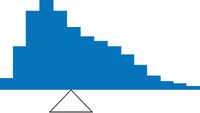
- This shows an asymmetric distribution.
- To balance it, we cannot put the fulcrum halfway between the lowest and highest values.
- Placing the fulcrum at the "half way" point would cause it to tip towards the left.
Smallest Absolute Deviation
- Another way to define the center of a distribution is based on the concept of the sum of the absolute deviations (differences).
- Consider the distribution made up of the five numbers 2, 3, 4, 9, 16.
- Let's see how far the distribution is from 10 (picking a number arbitrarily).
- Table below shows the sum of the absolute deviations of these numbers from the number 10.
| Values | Absolute Deviations from 10 |
|---|---|
| 2 | 8 |
| 3 | 7 |
| 4 | 6 |
| 9 | 1 |
| 16 | 6 |
| Sum | 28 |
- The first row of the table shows the absolute value of the difference between 2 and 10 is 8; the second row shows that the absolute difference between 3 and 10 is 7, and similarly for the other rows.
- When we add up the five absolute deviations, we get 28.
- So, the sum of the absolute deviations from 10 is 28.
- Likewise, the sum of the absolute deviations from 5 equals 3 + 2 + 1 + 4 + 11 = 21.
- So, the sum of the absolute deviations from 5 is smaller than the sum of the absolute deviations from 10.
- In this sense, 5 is closer, overall, to the other numbers than is 10.
- We are now in a position to define a second measure of central tendency, this time in terms of absolute deviations.
- Specifically, according to our second definition, the center of a distribution is the number for which the sum of the absolute deviations is smallest.
- As we just saw, the sum of the absolute deviations from 10 is 28 and the sum of the absolute deviations from 5 is 21.
- Is there a value for which the sum of the absolute deviations is even smaller than 21? Yes.
- For these data, there is a value for which the sum of absolute deviations is only 20.
Smallest Squared Deviation
- Smallest Squared Deviation is based on the concept of the sum of squared deviations (differences).
| Values | Absolute Deviations from 10 |
|---|---|
| 2 | 64 |
| 3 | 49 |
| 4 | 36 |
| 9 | 1 |
| 16 | 36 |
| Sum | 186 |
- Again, consider the distribution of the five numbers 2, 3, 4, 9, 16.
- Table above shows the sum of the squared deviations of these numbers from the number 10.
- The first row in the table shows the squared value of the difference between 2 and 10 is 64; the second row shows that the squared difference between 3 and 10 is 49, and so forth.
- When we add up all these squared deviations, we get 186.
- Changing the target from 10 to 5, we calculate the sum of the squared deviations from 5 as 9 + 4 + 1 + 16 + 121 = 151.
- So, the sum of the squared deviations from 5 is smaller than the sum of the squared deviations from 10.
- Is there a value for which the sum of the squared deviations is even smaller than 151? Yes, it is possible to reach 134.8.
- Can you find the target number for which the sum of squared deviations is 134.8?
- The target that minimizes the sum of squared deviations provides another useful definition of central tendency.
Quiz
Measures of Central Tendency
There are three most common measures of central tendency: the mean, the median, and the mode.
Arithmetic Mean
- the sum of the numbers divided by the number of numbers
- not the only "mean" (there is also a geometric mean), but the most commonly used to measure central tendency
- The symbol "μ" is used for the mean of a population.
- The symbol "M" is used for the mean of a sample.
The formula for μ is shown below:
μ = ΣX/N
where ΣX is the sum of all the numbers in the population and
N is the number of numbers in the population.
The formula for M is essentially identical:
M = ΣX/N
where ΣX is the sum of all the numbers in the sample and
N is the number of numbers in the sample.
For example, the mean of the numbers 1, 2, 3, 6, 8 is 20/5 = 4 regardless of whether the numbers constitute the entire population or just a sample from the population.
Median
- the 50th percentile
- the midpoint of a distribution: the same number of scores is above the median as below it.
Computation of the Median
- Odd number of numbers: the median is simply the middle number (the median of 2, 4, and 7 is 4).
- Even number of numbers: the median is the mean of the two middle numbers. (the median of 2, 4, 7, 12 is (4+7)/2 = 5.5).
- When there are numbers with the same values, then the formula for the third definition of the 50th percentile should be used.
Mode
- The mode is the most frequently occurring value.
- The mode of continuous data is normally computed from a grouped frequency distribution (since the frequency of each value is one since no two scores will be exactly the same).
| Range | Frequency |
|---|---|
| 500-600 | 3 |
| 600-700 | 6 |
| 700-800 | 5 |
| 800-900 | 5 |
| 900-1000 | 0 |
| 1000-1100 | 1 |
- Table above shows a grouped frequency distribution for the target response time data.
- Since the interval with the highest frequency is 600-700, the mode is the middle of that interval (650).
Quiz
Mean and Median
- the mean is the point on which a distribution would balance (Balance Scale)
- the median is the value that minimizes the sum of absolute deviations (Smallest Absolute Deviation)
- the mean is the value that minimizes the sum of the squared deviations (Smallest Squared Deviation)
| Value | Absolute Deviation from Median | Absolute Deviation from Mean | Squared Deviation from Median | Squared Deviation from Mean |
|---|---|---|---|---|
| 2 | 2 | 4.8 | 4 | 23.04 |
| 3 | 2 | 3.8 | 1 | 14.44 |
| 4 | 0 | 2.8 | 0 | 7.84 |
| 9 | 5 | 2.2 | 25 | 4.84 |
| 16 | 12 | 9.2 | 144 | 84.64 |
| Total | 20 | 22.8 | 174 | 134.8 |
- Table and figure above show the absolute and squared deviations of the numbers 2, 3, 4, 9, and 16 from their median of 4 and their mean of 6.8.
- The sum of absolute deviations from the median (20) is smaller than the sum of absolute deviations from the mean (22.8).
- The sum of squared deviations from the median (174) is larger than the sum of squared deviations from the mean (134.8).
When a distribution is symmetric, then the mean and the median are the same.
- Consider the following distribution: 1, 3, 4, 5, 6, 7, 9.
- The mean and median are both 5.
- The mean, median, and mode are identical in the bell-shaped normal distribution.
Quiz
Additional Measures of Central Tendency
- Although the mean, median, and mode are by far the most commonly used measures of central tendency, they are not the only measures.
- This section defines three additional measures of central tendency: the trimean, the geometric mean, and the trimmed mean.
Trimean
- The trimean is a weighted average of the 25th percentile, the 50th percentile, and the 75th percentile.
- The median is weighted twice as much as the 25th and 75th percentiles.
- Letting P25 be the 25th percentile, P50 be the 50th and P75 be the 75th percentile, the formula for the trimean is:
Trimean = (P25 + 2P50 + P75)/4
Example
37, 33, 33, 32, 29, 28, 28, 23, 22, 22,
22, 21, 21, 21, 20, 20, 19, 19, 18, 18,
18, 18, 16, 15, 14, 14, 14, 12, 12, 9, 6
- The box shows the number of touchdown (TD) passes thrown by each of the 31 teams in the National Football League.
- The relevant percentiles are shown in the table below.
| Percentile | Value |
|---|---|
| 25 | 15 |
| 50 | 20 |
| 75 | 23 |
The trimean is therefore (15 + 2 x 20 + 23)/4 = 78/4 = 19.5.
Geometric Mean
- The geometric mean is computed by multiplying all the numbers together and then taking the nth root of the product.
- The formula for the geometric mean is:
Example
- For the numbers 1, 10, and 100, the product of all the numbers is: 1 x 10 x 100 = 1,000.
- Since there are three numbers, we take the cubed root of the product (1,000) which is equal to 10.
(1 x 10 x 100 )1/3 = 10001/3 = 10
Geometric Meanand logarithms
- The geometric mean has a close relationship with logarithms.
- Table below shows the logs (base 10) of these three numbers.
- The arithmetic mean of the three logs is 1.
- The anti-log of this arithmetic mean of 1 is the geometric mean.
- The anti-log of 1 is 101 = 10.
- Note that the geometric mean only makes sense if all the numbers are positive.
| x | Log10(X) |
|---|---|
| 1 | 0 |
| 10 | 1 |
| 100 | 2 |
The geometric mean is an appropriate measure to use for averaging rates.
Example
- Consider a stock portfolio that began with a value of $1,000 and had annual returns of 13%, 22%, 12%, -5%, and -13%.
- Table below shows the value after each of the five years.
| Year | Return | Value |
|---|---|---|
| 1 | 13% | 1,130 |
| 2 | 22% | 1,379 |
| 3 | 12% | 1,544 |
| 4 | -5% | 1,467 |
| 5 | -13% | 1,276 |
- The question is how to compute average annual rate of return.
- The answer is to compute the geometric mean of the returns.
- Instead of using the percents, each return is represented as a multiplier indicating how much higher the value is after the year.
- This multiplier is 1.13 for a 13% return and 0.95 for a 5% loss.
- The multipliers for this example are 1.13, 1.22, 1.12, 0.95, and 0.87.
- The geometric mean of these multipliers is 1.05.
- Therefore, the average annual rate of return is 5%.
- Table below shows how a portfolio gaining 5% a year would end up with the same value ($1,276) as shown in above.
| Year | Return | Value |
|---|---|---|
| 1 | 5% | 1,050 |
| 2 | 5% | 1,103 |
| 3 | 5% | 1,158 |
| 4 | 5% | 1,216 |
| 5 | 5% | 1,276 |
Trimmed Mean
- To compute a trimmed mean, you remove some of the higher and lower scores and compute the mean of the remaining scores.
- A mean trimmed 10% is a mean computed with 10% of the scores trimmed off: 5% from the bottom and 5% from the top.
- A mean trimmed 50% is computed by trimming the upper 25% of the scores and the lower 25% of the scores and computing the mean of the remaining scores.
- The trimmed mean is similar to the median which, in essence, trims the upper 49+% and the lower 49+% of the scores.
- Therefore the trimmed mean is a hybrid of the mean and the median.
Example
- To compute the mean trimmed 20% for the touchdown pass data shown above, you remove the lower 10% of the scores (6, 9, and 12) as well as the upper 10% of the scores (33, 33, and 37) and compute the mean of the remaining 25 scores.
- This mean is 20.16.
Quiz
Comparing Measures of Central Tendency
- For symmetric distributions, the mean, median, trimean, and trimmed mean are equal, as is the mode except in bimodal distributions.
- Differences among the measures occur with skewed distributions.
Example 1
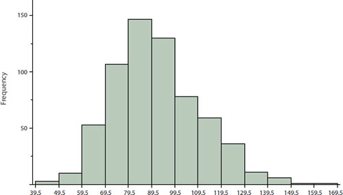
- Figure above shows the distribution of 642 scores on an introductory psychology test.
- Notice this distribution has a slight positive skew.
- Measures of central tendency are shown in the table below.
| Measure | Value |
|---|---|
| Mode | 84.00 |
| Median | 90.00 |
| Geometric Mean | 89.70 |
| Trimean | 90.25 |
| Mean trimmed 50% | 89.81 |
| Mean | 91.58 |
- Notice they do not differ greatly, with the exception that the mode is considerably lower than the other measures.
- When distributions have a positive skew, the mean is typically higher than the median, although it may not be in bimodal distributions.
- For these data, the mean of 91.58 is higher than the median of 90.
- Typically the trimean and trimmed mean will fall between the median and the mean, although in this case, the trimmed mean is slightly lower than the median.
- The geometric mean is lower than all measures except the mode.
Example 2
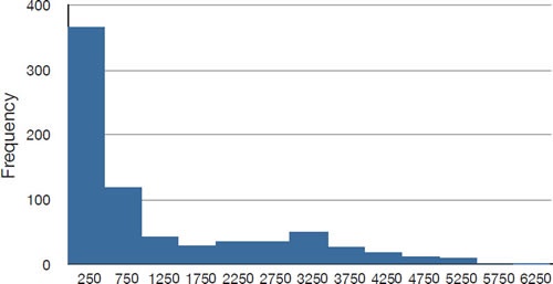
- The distribution of baseball salaries (in 1994) shown in the figure above has a much more pronounced skew than the distribution in Example 1.
- Table below shows the measures of central tendency for these data.
| Measure | Value |
|---|---|
| Mode | 250 |
| Median | 500 |
| Geometric Mean | 555 |
| Trimean | 792 |
| Mean trimmed 50% | 619 |
| Mean | 1,183 |
- The large skew results in very different values for these measures.
- No single measure of central tendency is sufficient for data such as these.
- If you were asked the very general question: "So, what do baseball players make?" and answered with the mean of $1,183,000, you would not have told the whole story since only about one third of baseball players make that much.
- If you answered with the mode of $250,000 or the median of $500,000, you would not be giving any indication that some players make many millions of dollars.
- Fortunately, there is no need to summarize a distribution with a single number.
- When the various measures differ, our opinion is that you should report the mean, median, and either the trimean or the mean trimmed 50%.
- Sometimes it is worth reporting the mode as well.
- In the media, the median is usually reported to summarize the center of skewed distributions.
- You will hear about median salaries and median prices of houses sold, etc.
- This is better than reporting only the mean, but it would be informative to hear more statistics.
Quiz
<quiz display=simple >
{ When reporting the central tendency of a highly skewed distribution, you should report:
|type="()"} -Mean -Median -Mode -Trimean -Mean trimmed 50% +More than one of the above
{
Answer >>
More than one of the above
One of these measures does not summarize a skewed distribution well. It is good to report multiple statistics such as median, mean, and trimean.
}
{ Which of these measures of central tendency is most likely to be very different from the rest?
|type="()"} -Mean -Median +Mode -Trimean -Mean trimmed 50%
{
Answer >>
Mode
Although differences among all the measures occur with skewed distributions, the mode is generally the most likely to be very different than the rest. For example, if there is a bimodal distribution, there could be two modes, one a lot higher and one a lot lower than the mean and median. Even in the slightly skewed psychology test score data presented in Figure 1 and Table 1, the mode is a lot lower than the other measures of central tendency because the most common score happened to be far below the center.
}
{When a distribution has a positive skew, what is the relationship between the median and the mean?
|type="()"} +Mean greater than Median -Mean less than Median -Mean = Median
{
Answer >>
Mean greater than Median
A distribution with a positive skew has a longer tail to the right of the distribution, and the mean is higher than the median.
}

